Exploratory Data Analysis with R
With this RMarkdown document we will present some basic methods to overview given data.
The required R Packages are:
require(tidyverse)   # tidyverse is the sine qua non, see https://www.tidyverse.org/ and includes important packages like tidyr, dplyr, ggplot2, readr, magrittr etc
require(skimr)  # skimr creates nice overview tables and does with dplyr and piping
require(mosaic)  # mosaic includes also ggformula and lattice packages
require(QuantPsyc)   # QuantPsyc delivers useful statistical functions like "Make.Z" and "eda.uni"
Get the full glimpse
We will use the fancy starwars dataframe from {dplyr} package, and call it sw for the sake of convenience.
sw <- starwars   # copy to "sw"
sw   # just view
For plain R output there is a concise first viewing option of a dataframe with the glimpse command.
glimpse(sw)
## Rows: 87
## Columns: 14
## $ name       <chr> "Luke Skywalker", "C-3PO", "R2-D2", "Darth Vader", "Leia...
## $ height     <int> 172, 167, 96, 202, 150, 178, 165, 97, 183, 182, 188, 180...
## $ mass       <dbl> 77.0, 75.0, 32.0, 136.0, 49.0, 120.0, 75.0, 32.0, 84.0, ...
## $ hair_color <chr> "blond", NA, NA, "none", "brown", "brown, grey", "brown"...
## $ skin_color <chr> "fair", "gold", "white, blue", "white", "light", "light"...
## $ eye_color  <chr> "blue", "yellow", "red", "yellow", "brown", "blue", "blu...
## $ birth_year <dbl> 19.0, 112.0, 33.0, 41.9, 19.0, 52.0, 47.0, NA, 24.0, 57....
## $ sex        <chr> "male", "none", "none", "male", "female", "male", "femal...
## $ gender     <chr> "masculine", "masculine", "masculine", "masculine", "fem...
## $ homeworld  <chr> "Tatooine", "Tatooine", "Naboo", "Tatooine", "Alderaan",...
## $ species    <chr> "Human", "Droid", "Droid", "Human", "Human", "Human", "H...
## $ films      <list> [<"The Empire Strikes Back", "Revenge of the Sith", "Re...
## $ vehicles   <list> [<"Snowspeeder", "Imperial Speeder Bike">, <>, <>, <>, ...
## $ starships  <list> [<"X-wing", "Imperial shuttle">, <>, <>, "TIE Advanced ...
There are 14 variables, of which 3 are a list type. The other variables are numbers or characters, last ones partly better to be transformed into categorical (i.e. factor or dummy) variables.
Before we transform them, we might look at their unique values. Also "NA"s, R's term for non-existent values, are printed.
# show unique values for the specified variable, here columns 9, "gender" and 4, "hair_color" - which indeed is a tiny example of a for-loop
for (i in c(9,4)) {
       unique(sw[,i]) %>% print.AsIs()
}
##      gender
## 1 masculine
## 2  feminine
## 3      <NA>
##       hair_color
## 1          blond
## 2           <NA>
## 3           none
## 4          brown
## 5    brown, grey
## 6          black
## 7  auburn, white
## 8   auburn, grey
## 9          white
## 10          grey
## 11        auburn
## 12        blonde
## 13       unknown
We might notice that there are 2 different "blond/blonde" values in hair_color. Let's change this!
We'll use the pipe %>% formula as we take the sw dataframe, do the mutation and write it back to sw.
Second, we turn hair_color into a factor variable.
sw <- sw %>% mutate(hair_color = replace(hair_color, which(hair_color=="blonde"), "blond"))
sw$hair_color <- as.factor(sw$hair_color)
Here's one more, very concise overview option (also using the pipe formula) -- which may help best at large datasets.
skim(sw) %>% summary()
Table: Data summary
| Name | sw |
| Number of rows | 87 |
| Number of columns | 14 |
| _____ | |
| Column type frequency: | |
| character | 7 |
| factor | 1 |
| list | 3 |
| numeric | 3 |
| ______ | |
| Group variables | None |
Before continue with overview statistics we might get clear about adressing and accessing parts of the dataframe. So-called subsetting a dataframe in R ist quite easy to do, you just need to adress the relevant rows and/or columns by numbers in squared brackets, and use the vector format c(x,y,z) for multiple ones. (Of course there are more elaborate options to do this, but for now we stick to shortness and the usage in the functions beneath.)
sw[1:5, c(1,6:4)] # first 5 rows of columns 1, 6, 5, 4
sw[3, -c(5:ncol(sw))] # row 3 with columns 1 to 4 by sorting out columns 5 to the last
Let's now get a better insight into certain variables. For this we use the skim function from the package {skimr}. (Of course you can also "skim" the whole dataframe if you want to: It might deliver a large table, anyway.) skim gives us very useful basic statistics for the chosen variables according to their type, and even a mini histogram where appropriate.
Therefore, skim is very useful at checking for missing values (and their share), whitespaces and unique values, and also a first glimpse of the single variate distributions.
# skimming a character, numerical, integer, factor variable
skim(sw, sex, birth_year, height, hair_color)   # alternatively use column numbers like "skim(sw, c(8, 7, 2, 4))"
Table: Data summary
| Name | sw |
| Number of rows | 87 |
| Number of columns | 14 |
| _____ | |
| Column type frequency: | |
| character | 1 |
| factor | 1 |
| numeric | 2 |
| ______ | |
| Group variables | None |
Variable type: character
| skim_variable | n_missing | complete_rate | min | max | empty | n_unique | whitespace |
|---|---|---|---|---|---|---|---|
| sex | 4 | 0.95 | 4 | 14 | 0 | 4 | 0 |
Variable type: factor
| skim_variable | n_missing | complete_rate | ordered | n_unique | top_counts |
|---|---|---|---|---|---|
| hair_color | 5 | 0.94 | FALSE | 11 | non: 37, bro: 18, bla: 13, blo: 4 |
Variable type: numeric
| skim_variable | n_missing | complete_rate | mean | sd | p0 | p25 | p50 | p75 | p100 | hist |
|---|---|---|---|---|---|---|---|---|---|---|
| birth_year | 44 | 0.49 | 87.57 | 154.69 | 8 | 35 | 52 | 72 | 896 | ▇▁▁▁▁ |
| height | 6 | 0.93 | 174.36 | 34.77 | 66 | 167 | 180 | 191 | 264 | ▁▁▇▅▁ |
We also turn the other appropriate variables into factors and may check with glimpse one more time.
sw[,c(5:6,8:11)] <- lapply(sw[,c(5:6,8:11)], as.factor)   # turning columns 5, 6 and 8 to 11 into factors
glimpse(sw)
## Rows: 87
## Columns: 14
## $ name       <chr> "Luke Skywalker", "C-3PO", "R2-D2", "Darth Vader", "Leia...
## $ height     <int> 172, 167, 96, 202, 150, 178, 165, 97, 183, 182, 188, 180...
## $ mass       <dbl> 77.0, 75.0, 32.0, 136.0, 49.0, 120.0, 75.0, 32.0, 84.0, ...
## $ hair_color <fct> "blond", NA, NA, "none", "brown", "brown, grey", "brown"...
## $ skin_color <fct> "fair", "gold", "white, blue", "white", "light", "light"...
## $ eye_color  <fct> blue, yellow, red, yellow, brown, blue, blue, red, brown...
## $ birth_year <dbl> 19.0, 112.0, 33.0, 41.9, 19.0, 52.0, 47.0, NA, 24.0, 57....
## $ sex        <fct> male, none, none, male, female, male, female, none, male...
## $ gender     <fct> masculine, masculine, masculine, masculine, feminine, ma...
## $ homeworld  <fct> Tatooine, Tatooine, Naboo, Tatooine, Alderaan, Tatooine,...
## $ species    <fct> Human, Droid, Droid, Human, Human, Human, Human, Droid, ...
## $ films      <list> [<"The Empire Strikes Back", "Revenge of the Sith", "Re...
## $ vehicles   <list> [<"Snowspeeder", "Imperial Speeder Bike">, <>, <>, <>, ...
## $ starships  <list> [<"X-wing", "Imperial shuttle">, <>, <>, "TIE Advanced ...
Inspect a subset
We might take a look at a specific subset of the whole dataset.
With base R sapply there is a single command to apply the same function to several variables or the whole dataframe.
sapply(sw[,c(4:6,8:11)], nlevels) # number of levels for the categoricals (columns 4 to 6 and 8 to 11)
## hair_color skin_color  eye_color        sex     gender  homeworld    species
##         11         31         15          4          2         48         37
sapply(sw[,2:3], median, na.rm=T) # median score for the numericals (columns 2 and 3); "na.rm" for ignoring the NA's
## height   mass
##    180     79
The function select from {dplyr} offers a kind way of including or excluding variables, which pays off best using it in building a data pipe. After selecting you can continue with various statistical functions like summary here.
sw %>% dplyr::select(-c(name,films, vehicles, starships, c(4:7))) %>%    # exclude certain variables
  summary()     # statistical summaries for the left variables
##      height           mass                     sex           gender
##  Min.   : 66.0   Min.   :  15.00   female        :16   feminine :17
##  1st Qu.:167.0   1st Qu.:  55.60   hermaphroditic: 1   masculine:66
##  Median :180.0   Median :  79.00   male          :60   NA's     : 4
##  Mean   :174.4   Mean   :  97.31   none          : 6
##  3rd Qu.:191.0   3rd Qu.:  84.50   NA's          : 4
##  Max.   :264.0   Max.   :1358.00
##  NA's   :6       NA's   :28
##      homeworld      species
##  Naboo    :11   Human   :35
##  Tatooine :10   Droid   : 6
##  Alderaan : 3   Gungan  : 3
##  Coruscant: 3   Kaminoan: 2
##  Kamino   : 3   Mirialan: 2
##  (Other)  :47   (Other) :35
##  NA's     :10   NA's    : 4
Looking at individual variables
The tiny str command will generally check of which type or structure a variable or any R object is, with it's sibling summary it is also used beyond EDA.
str(sw$sex)
## Factor w/ 4 levels "female","hermaphroditic",..: 3 4 4 3 1 3 1 4 3 3 ...
str(sw$name)
## chr [1:87] "Luke Skywalker" "C-3PO" "R2-D2" "Darth Vader" "Leia Organa" ...
str(sw$birth_year)
## num [1:87] 19 112 33 41.9 19 52 47 NA 24 57 ...
Numerical (continuous) variables
For numerical variables there are dedicated statistical commands like:
summary(sw$birth_year)
##    Min. 1st Qu.  Median    Mean 3rd Qu.    Max.    NA's
##    8.00   35.00   52.00   87.57   72.00  896.00      44
range(sw$birth_year, na.rm=T) # note another option for dealing with NA's
## [1] 8 896
quantile(sw$height, probs=0.8, na.rm=T) # 8th quantile
## 80%
## 193
top_counts(sw$height, max_levels=5) # top 5 values with counts
## [1] "183: 7, 180: 5, 188: 5, 170: 4, 178: 4"
Also, there are options which deliver the numbers in particular output formats, like skim we already know. df_stats from the {ggformula} package creates a dataframe, and can also be adapted.
skim(sw$birth_year) # for further options with skim see above
Table: Data summary
| Name | sw$birth_year |
| Number of rows | 87 |
| Number of columns | 1 |
| _____ | |
| Column type frequency: | |
| numeric | 1 |
| ______ | |
| Group variables | None |
Variable type: numeric
| skim_variable | n_missing | complete_rate | mean | sd | p0 | p25 | p50 | p75 | p100 | hist |
|---|---|---|---|---|---|---|---|---|---|---|
| data | 44 | 0.49 | 87.57 | 154.69 | 8 | 35 | 52 | 72 | 896 | ▇▁▁▁▁ |
df_stats(~ mass, data=sw) # standard view by df_stats
df_stats(~ mass, data=sw, quantile, iqr, mad) # adapted df_stats output
## Warning: Excluding 28 rows due to missing data [df_stats()].
Turning numerical values into standard normal values can be done in a quite a simple way using the Make.Z command, or alternatively with scale. Both can be also applied on whole dataframes.
sw$heightZ <- Make.Z(sw$height)   # converting into z-scores (standard-normal)
sw$massZ <- scale(sw$mass)  # same for mass, with scale()
# as.data.frame(Make.Z(x))   # back converting into dataframe, when Make.Z is applied to a whole dataframe
Categorical (factor) variables
For factor variables there are several ways for inspecting them.
summary(sw$gender) # levels with counts, with NA's
##  feminine masculine      NA's
##        17        66         4
mosaic::tally(~gender, data=sw) # gives a nice print out
## gender
##  feminine masculine      <NA>
##        17        66         4
levels(sw$gender) # only levels, without counts, without NA's
## [1] "feminine" "masculine"
skim(sw$gender) # for further options with skim see above
Table: Data summary
| Name | sw$gender |
| Number of rows | 87 |
| Number of columns | 1 |
| _____ | |
| Column type frequency: | |
| factor | 1 |
| ______ | |
| Group variables | None |
Variable type: factor
| skim_variable | n_missing | complete_rate | ordered | n_unique | top_counts |
|---|---|---|---|---|---|
| data | 4 | 0.95 | FALSE | 2 | mas: 66, fem: 17 |
Why it is worth knowing various of them? For instance, you can use them to address particular data.
levels(sw$gender)[1]
## [1] "feminine"
summary(sw$gender)[3]
## NA's
##    4
For combining in 2 factor variables into a cross table you can use table or the tally command from {mosaic} package -- they differ in handling the NA's.
table(sw$gender, sw$sex) # crosstable with NA's being ignored; more options are available with xtabs()
##
##             female hermaphroditic male none
##   feminine      16              0    0    1
##   masculine      0              1   60    5
mosaic::tally(gender ~ sex, data=sw) # crosstable including NA's
##            sex
## gender      female hermaphroditic male none <NA>
##   feminine      16              0    0    1    0
##   masculine      0              1   60    5    0
##   <NA>           0              0    0    0    4
There is also a way to have an insight of the distribution of factor variables using the top_levels command from the {janitor} package.
Note how we use a command from a package NOT sourced in this R/RMarkdown script -- that's a stunning feature of R.
janitor::top_levels(sw$eye_color, n=3, show_na=T) # n = number in top & bottom group
Remember skim above? Of course you can use skim for inspecting a single variable. But you can even adjust skim to your own needs. Just write a small function with the skim_with command like "my_skim" with MAD, IQR and 10th quantile here.
my_skim <- skim_with(
  numeric = sfl(mad = mad, iqr = IQR, p10 = ~ quantile(., probs = .1)), append = F)
# my_skim(sw$mass)  # What's the problem here?
Different R functions ignore or don't ignore NA's in calculating, as we might have seen. Often bug fixing is just to take NA's explicitly into account, for instance with the na.omit command.
my_skim(na.omit(sw$mass))
Table: Data summary
| Name | na.omit(sw$mass) |
| Number of rows | 59 |
| Number of columns | 1 |
| _____ | |
| Column type frequency: | |
| numeric | 1 |
| ______ | |
| Group variables | None |
Variable type: numeric
| skim_variable | n_missing | complete_rate | mad | iqr | p10 |
|---|---|---|---|---|---|
| data | 0 | 1 | 16.31 | 28.9 | 44 |
Grouped variables statistics
The {dplyr} function group_by easily splits the dataframe into groups along certain variables (factors and numerical!) and works fine with the pipe.
sw %>% dplyr::group_by(gender) %>%    # building groups by gender
    dplyr::select(c(2:4))   %>%     # reducing the output by select only a few columns
         skim()     # skim overview according to the gender groups
## Adding missing grouping variables: `gender`
Table: Data summary
| Name | Piped data |
| Number of rows | 87 |
| Number of columns | 4 |
| _____ | |
| Column type frequency: | |
| factor | 1 |
| numeric | 2 |
| ______ | |
| Group variables | gender |
Variable type: factor
| skim_variable | gender | n_missing | complete_rate | ordered | n_unique | top_counts |
|---|---|---|---|---|---|---|
| hair_color | feminine | 0 | 1.00 | FALSE | 6 | bro: 6, non: 5, bla: 3, aub: 1 |
| hair_color | masculine | 5 | 0.92 | FALSE | 9 | non: 31, bro: 11, bla: 9, blo: 3 |
| hair_color | NA | 0 | 1.00 | FALSE | 4 | bla: 1, bro: 1, non: 1, unk: 1 |
Variable type: numeric
| skim_variable | gender | n_missing | complete_rate | mean | sd | p0 | p25 | p50 | p75 | p100 | hist |
|---|---|---|---|---|---|---|---|---|---|---|---|
| height | feminine | 1 | 0.94 | 164.69 | 23.55 | 96 | 161.50 | 165.5 | 172.0 | 213 | ▁▁▇▆▁ |
| height | masculine | 4 | 0.94 | 176.52 | 37.65 | 66 | 171.25 | 183.0 | 193.0 | 264 | ▂▁▇▇▁ |
| height | NA | 1 | 0.75 | 181.33 | 2.89 | 178 | 180.50 | 183.0 | 183.0 | 183 | ▃▁▁▁▇ |
| mass | feminine | 8 | 0.53 | 54.69 | 8.59 | 45 | 50.00 | 55.0 | 56.2 | 75 | ▇▇▁▁▂ |
| mass | masculine | 17 | 0.74 | 106.15 | 184.97 | 15 | 75.00 | 80.0 | 88.0 | 1358 | ▇▁▁▁▁ |
| mass | NA | 3 | 0.25 | 48.00 | NA | 48 | 48.00 | 48.0 | 48.0 | 48 | ▁▁▇▁▁ |
We've already heard about the df_stats for single variables. Bit it's also very useful for variables grouped by another, as here height by gender groups. Note that NA's are ignored by default.
df_stats(height ~ gender, data=sw) # standard view by df_stats
And this works for grouping along continuous variables, too -- and of course with specifying the statistical values.
df_stats(height ~ mass, data=sw, mean, range) # mean and range of height by mass "classes"
## Warning: Excluding 28 rows due to missing data [df_stats()].
Plots
Numbers are fine, but one should always take a look at plots where possible. Note that the plotting options presented here are not primarily meant for a beautiful data visualisation, but for inspecting the given data.
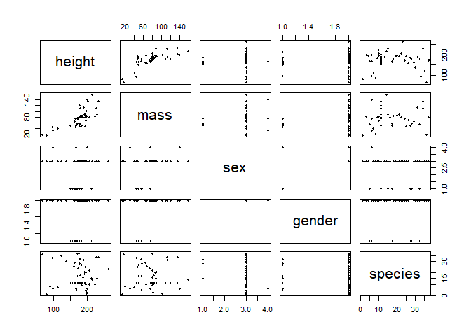
The easiest way to get a picture of possible correlations ist to use plot on the whole dataframe or the variables to take into account. Here, we chose to check height, mass, sex, gender and species, and dropped the 16th observation, which is "Jabba the Hutt", presumably an outlier with his exceptional body shape.
plot(sw[-16,c(2,3,8,9, 11)], pch=20) # "pch" sets the shape of the points; alternatively use "pairs"
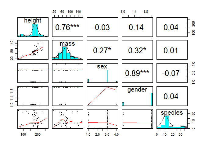
pairs.panels from the {psych} package is a more elaborative form of it, including correlation scores and various output/layout options. These may help especially when inspecting more variables at once, for instance by starring or scaling up the font of high correlation coefs.
psych::pairs.panels(sw[-16,c(2,3,8,9, 11)], method = "pearson", density=T, stars=T, ellipses=F) # also available: spearman and kendall correlation
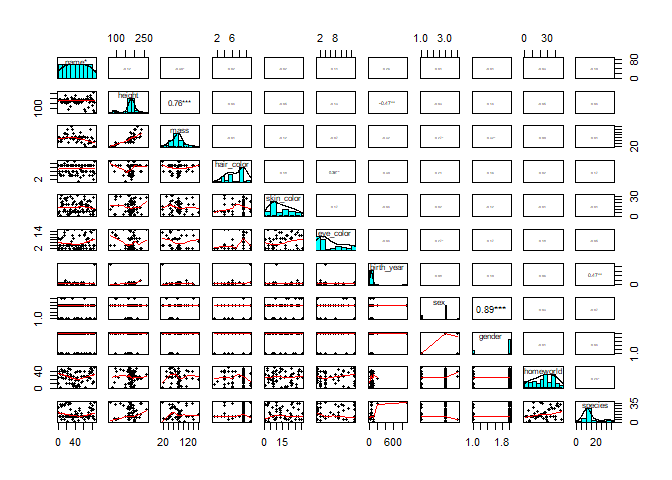
psych::pairs.panels(sw[-16,1:11], method = "pearson", density=T, scale=T, ellipses=F, stars=T)
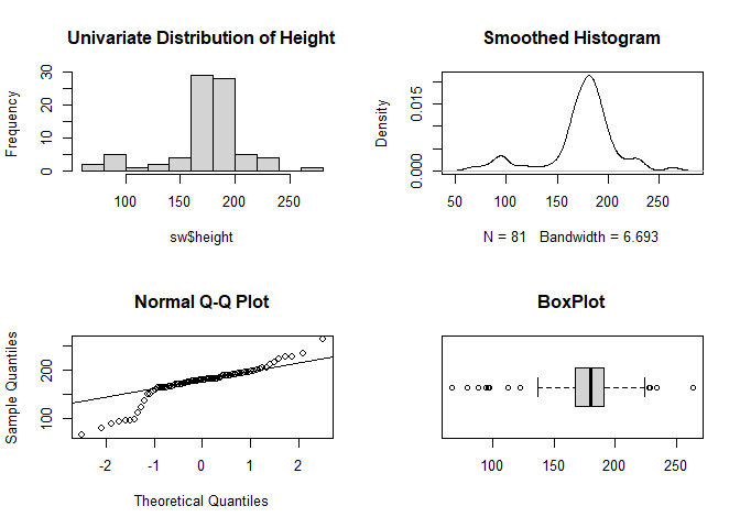
The eda.uni function in {QuantPsyc} is a good start for inspecting univariate distributions, as it combines four relevant plots: histogram, density plot, normal plot and boxplot.
eda.uni(sw$height, title="Univariate Distribution of Height") # 4 plots in one :)
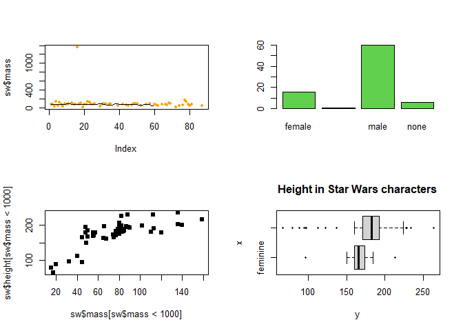
There are various plot options, which can be parametrised in numerous ways. plot as the simplest of them will adjust to the given variable type/types.
par(mfrow=c(2,2))   # sets visual parameter for showing the following plots in a 2x2 grid pattern
plot(sw$mass, pch=20, col="orange"); lines(smooth(na.omit(sw$mass)))   # smooth = Tukey's (running median) smoothing; writing 2 lines of code into one by separating them with ";"
plot(sw$sex, col=3)  # colour can also be given as integer
plot(sw$mass[sw$mass < 1000], sw$height[sw$mass < 1000], pch=15)   # with subsetting the data; "pch" parameter refers to the shape of points
plot(sw$gender, sw$height, pch=20, main="Height in Star Wars characters", horizontal=T)
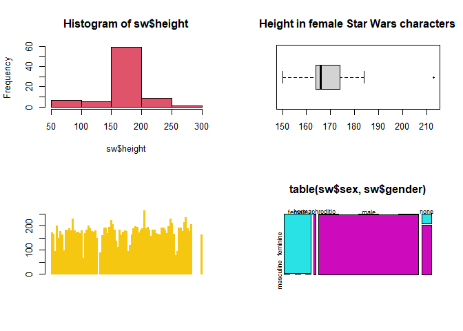
Certain plots can be addressed by basic commands like hist, boxplot, barplot or mosaicplot.
par(mfrow=c(2,2))
hist(sw$height, breaks=5, col=18)    # with given number of bins
boxplot(sw$height[sw$sex=="female"], horizontal = T, pch=20, main="Height in female Star Wars characters")   # with female sex filter
barplot(sw$height, col=7, border=7)   # border sets the colour of the shape margins
mosaicplot(table(sw$sex, sw$gender), col=5:6)
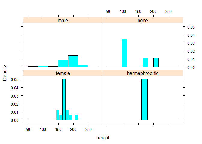
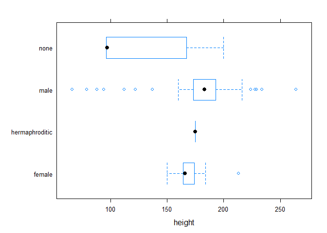
histogram and bwplot from the {lattice} package offer easy plots for grouped variables.
Note that adressing a function with its full package name like package::command makes sure to get the right command if there are homonymous ones.
lattice::histogram(~height|sex, data=sw) # histogram of height by sex groups
lattice::bwplot(sex~height, data=sw) # boxplot of height by sex groups
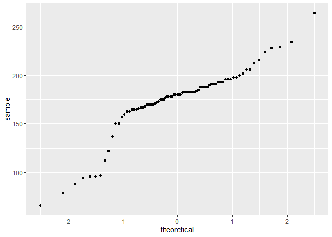
As noted before there are far more elaborate options to plot data, first and foremost with the {ggplot2} package. We won't dive into this, but give a short view on it by using the {ggfomula} shortcuts for it. With their shortened grammar there are also a good compromise between quickness and nice view for EDA.
# further ggformula plots are for instance gf_histogram(), gf_dens(), gf_freqpoly(), gf_dotplot(), gf_bar(), gf_violin, along several layout options
gf_qq(~ height, data=sw)     # normal plot for height
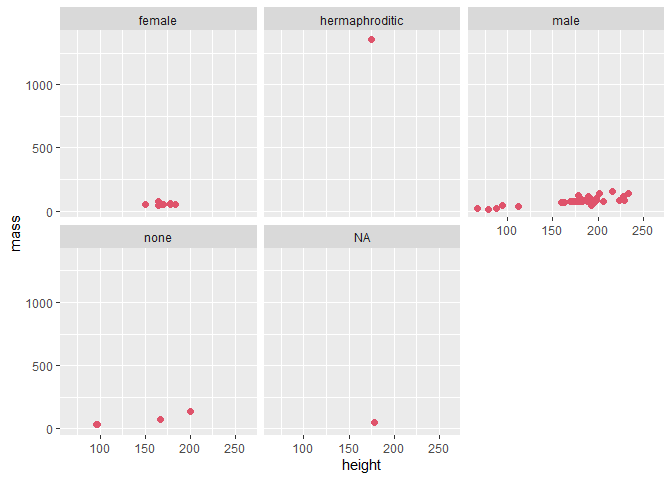
gf_point(mass ~ height | sex, data=sw, size=2, col=2) # height vs. mass grouped by sex
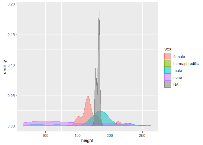
gf_density(~ height, colour=~sex, data=sw, alpha=0.5, fill=~sex) # density plot for height gouped by sex
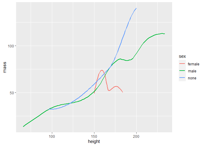
gf_smooth(mass ~ height, color=~sex, data=sw, size = 1) # loess is standard smoothing method